Hybrid Monte Carlo Sampling for Bayesian Logistic Regression

Main Page

Contents

Load data

The variable 'data' is returned as a struct with covariates X of size NxD and labels Y of size Nx1.

setSeed(1);
[dataDir, outDir] = setupDir;

data = getBinData('ripley', dataDir);
[N, D] = size(data.X);

Hyperparameters

Hypers should be a struct with any hyperparameters needed for the model. Also useful to send the dimensions of the data. These dimensions are useful for models such as Factor Analysis where we must also specify the number of latent dimensions. Also, where we are sampling more than one parameter (e.g., again factor analysis, sampling both factor and coefficients), these dimensions allow us to index correctly.

hypers.dims.N = N;
hypers.dims.D = D;
hypers.alpha = 1;

HMC Settings

Specify a log probability function, which return the the joint probability and the first derivative with respect to all parameters that are to be sampled.

logprob = @bayesLogReg;

nSamples = 200;
burnin = 100;

% These are parameters to set for HMC
options = struct(...
    'nSamples', nSamples, ...
    'nLeaps',  200, ...
    'stepSize', 0.1, ...
    'display',0);

Initialisation

Here we add one dimension for the bias term.

options.initVec = rand(D+1,1);

Running HMC

disp('Running HMC ...');
[samples, stats] = hmc(logprob, data, hypers, options);

Running HMC ...

HMC Complete

Posterior Analysis

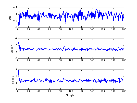
1. Trace Plots examining the bias and params.

figure;
subplot(3,1,1);
plot(samples(:,1), 'LineWidth',2);
ylabel('Bias');
subplot(3,1,2)
plot(samples(:,2), 'LineWidth',2);
ylabel('Slope 1');
subplot(3,1,3)
plot(samples(:,3), 'LineWidth',2);
ylabel('Slope 2'); xlabel('Sample');
snapnow;

2. Effective Sample Size

ESS = CalculateESS(samples(burnin+1:end,:), nSamples - burnin -1);
disp('ESS Values: [bias slope1 slope2]');
disp(ESS);

ESS Values: [bias slope1 slope2]
       91.037          100       81.595

3. Compare Parameter Estimates

betaMean = mean(samples);
B = mnrfit(data.X,data.Y+1);
disp({'Post Mean', 'Max Lik'})
disp([betaMean' -B])

    'Post Mean'    'Max Lik'

     -0.11374     -0.12281
      0.80188      0.89296
       2.6634       2.9799

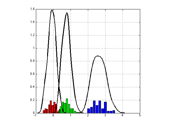
4. Parameter Histograms

figure;
col = getColorsRGB;
for i = 1:size(samples,2)
    % subplot(1,3,i);
    [n, xout] = hist(samples(burnin+1:end,i));
    bar(xout,n./sum(n),'FaceColor',col(i,:));
    axis square; hold on;
    [f, xi] = ksdensity(samples(burnin+1:end,i));
    plot(xi,f,'LineWidth',2,'Color','k');
    grid on;
end;
snapnow;

Shakir Mohamed, 2012

Published with MATLAB® 7.12