Exponential Family Factor Analysis

Main Page

Generate samples for exponential family factor analysis using Hybrid Monte Carlo sampling.

Contents

Model Setup

Specify the data to use and the number of latent factors K. We generate 5000 samples. All HMC settings are specified in the configuration file.

dataName = 'synth';
model = 'efa';
K = 3;
seed = 1;

[dataDir, outDir] = setupDir;
fileName = sprintf([outDir '/%s/%s_%s_%d'], dataName,model, 'hmc', K);

options = getConfigEFLVM(dataName, model);
burnin = options.burnin;
thin = options.thin;
saveOut = options.saveout;
setSeed(seed);

Load Data

dat = getBinData(dataName, dataDir);
[N,D] = size(dat.trueX);

Run EFA

Load a previously stored results if available

disp('Running HMC ...');
if ~exist([fileName,'.mat'],'file')
    %exptEFLVM(dataName,model,K, seed);
    inferFun = @inferEFA_hmc;
    predFun = @predProbEFA_mcmc;

    % Run HMC for few steps
    postDist = inferFun(dat, options, K);

    % Save
    if saveOut, save(fileName, 'postDist', 'seed'); end

    % Test error
    if isfield(dat,'miss')
        % only test if testing data exists
        [teErr, rmse, pHat] = predFun(dat, postDist.samples, K, burnin, thin);
        if saveOut, save(fileName,'teErr', 'rmse','-append'); end;
    end;
end;

res = load(fileName);

Running HMC ...

Posterior Analysis

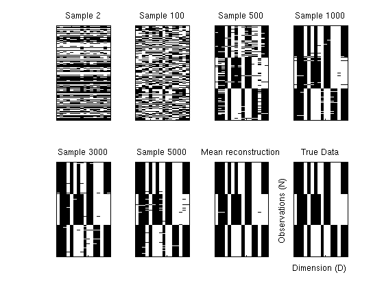
Plot reconstructions as the sampler progresses to show learning behaviour.

figure;
ix = [2, 100, 500, 1000,3000, 5000];
% Reconstructions for various samples
for i = 1:length(ix)
    [V, Theta , ~, ~] = extractParams(res.postDist.samples(ix(i),:), D, N, K);
    pStar = V*Theta;
    recon = 1./(1 + exp(-pStar))';
    subplot(2,4,i);
    imagesc(recon'> 0.5);
    title(sprintf('Sample %d',ix(i)));
    set(gca,'xticklabel',[],'yticklabel',[]);
    colormap gray;
end;

% Mean reconstruction
pStar = zeros(N,D);
rng = 3000:30:5000;
for i = rng
    [V, Theta , ~, ~] = extractParams(res.postDist.samples(i,:), D, N, K);
    pStar = pStar + V*Theta;
end;
pStar = pStar./length(rng);
recon = 1./(1 + exp(-pStar))';
subplot(2,4,7);
imagesc(recon'>0.5);
title('Mean reconstruction');
set(gca,'xticklabel',[],'yticklabel',[]);

% Noise free data
subplot(2,4,8);
imagesc(dat.cleanX);
title('True Data');
set(gca,'xticklabel',[],'yticklabel',[]);
ylabel('Observations (N)');
xlabel('Dimension (D)')
snapnow

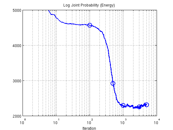
2. Plot Energy (negative log joint probability using training data)

figure;
semilogx(res.postDist.energy,'b-','LineWidth',2);
ylim([2000 5000]);
set(gca,'ytick',[2000:1000:5000]);
set(gca,'xtick',[10.^([0:4])])
title('Log Joint Probability (Energy)');
xlabel('Iteration');
grid on;
hold on;
plot(ix,res.postDist.energy(ix),'o','LineWidth',2,'MarkerSize',12);

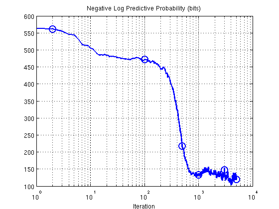
3. Predictive probability (bits) as sampler progresses

S = size(res.postDist.samples,1);
teErr = []; rmse = [];
for i = 1:S
    [teErr(i), rmse(i), ~] = predProbEFA_mcmc(dat, res.postDist.samples(i,:), K, 1, 1);
end;
figure;
semilogx(teErr,'b-','LineWidth',2)
% ylim([-200 600]);
% set(gca,'ytick',[-200:200:600], 'yticklabel',[-200:200:600]);
set(gca,'xtick',[10.^([0:4])])
title('Negative Log Predictive Probability (bits)');
xlabel('Iteration');
grid on;
hold on;
plot(ix,teErr(ix),'o','LineWidth',2,'MarkerSize',12);

Shakir Mohamed, 2012

Published with MATLAB® 7.14